Like racecars on a track, thousands of particles called muons zip around an experiment’s giant 50-foot circular magnet at 99.9% of the speed of light. After making a few hundred laps in less than a millisecond, the muons decay and are soon replaced by another bunch.
The goal of the experiment, Fermilab Muon g-2, is to better understand the properties of muons, which are essentially heavier versions of electrons, and use them to probe the limitations of the Standard Model of particle physics. Specifically, physicists want to know about the muons’ “magnetic moment”—that is, how much do they rotate on their axes in a powerful magnetic field— as they race around the magnet?
In 2001, an experiment at the US Department of Energy’s Brookhaven National Lab found that the muons turned more than theory predicted. The result surprised the physics community: If there really were a discrepancy, it could be a hint of new physics, like some as-yet-unknown particle influencing the muon. Two decades later, physicists hope to resolve the matter. Fermilab Muon g-2 aims to quadruple the precision of the 2001 finding and determine whether experiment really disagrees with theory.
There’s another side to the search though—one that’s carried out not with particle accelerators and giant magnets, but with equations on blackboards and computer simulations. Since 2016, another group of physicists has been trying to update the theoretical prediction of the muon’s magnetic moment by combining the efforts of several groups.
In June, the Muon g-2 Theory Initiative, which comprises 132 physicists across 82 institutions, published its first prediction: They calculated the muon’s anomalous magnetic moment, or αµ, to be 116,591,810x10-11. The value differs subtly, but significantly from the 2001 experiment, which found αµ to be 116,592,089x10-11. (That’s a difference of less than 3 parts per million, for those keeping score at home.)
“This is the first time that the entire community has come together and reached a consensus on the Standard Model prediction of this quantity,” says Aida X. El-Khadra, a physicist at the University of Illinois Urbana-Champaign and cofounder of the Theory Initiative. Previously, individual groups produced their own predictions of αµ, which differed slightly from one another.
By combining their efforts, physicists in the Theory Initiative hope that they’ll be able to come up with an ultra-precise prediction to complement the forthcoming result from the Fermilab Muon g-2 experiment. Both the experiment and the theory initiative receive support from DOE’s Office of Science.
But just how do physicists predict something like the muon’s magnetic moment, and why does it take 132 of them?
The path to g-2
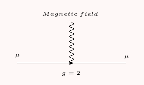
The first calculations of particle magnetic moments came in the 1920s, when physicists were just beginning to develop relativistic quantum mechanics. British theoretical physicist Paul Dirac, building on the work of Llewellyn Thomas and others, found the ultimate equation describing the electron and its spin—then conceived of as the electron’s internal rotation—and its magnetic moment. Dirac predicted this number, called “g,” to be exactly 2.
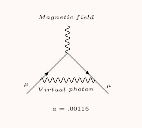
But atomic spectroscopy experiments soon found that g differed from that prediction by about 0.1%—a so-called “anomalous” magnetic moment, αe. In 1947, Julian Schwinger developed a theoretical explanation: The electron could emit and then reabsorb a virtual photon, which slightly changed its interaction with a magnetic field.
“Every way that something can happen in nature will happen,” says Tom Blum, a theoretical physicist at the University of Connecticut. “If a particle starts from here and gets to there, it can take all possible paths to get from there to there. And what quantum field theory tells us is how to weight those paths.”
The emission and absorption of a single virtual photon is just the most straightforward of these possible particle paths. Since Schwinger, physicists have been working to calculate increasingly unlikely possible paths that a particle can take. Ironically, the way they think about these paths is with a tool of Schwinger’s rival, Richard Feynman. To illustrate the paths and calculate their probabilities, Feynman developed his eponymously named diagrams.
Here, the Feynman diagram represents a muon (the Greek letter mu) moving left to right in a magnetic field (the squiggly line, which also denotes a photon).
The Feynman diagram for Schwinger’s path is slightly more complicated—this time there’s a squiggly blue line, the virtual photon being emitted and absorbed by the muon. This contributes approximately 0.00116 to αµ. This is the vast majority of muon’s anomalous magnetic moment.
To make the task manageable, the Theory Initiative segmented the task of calculating the muon’s magnetic moment into each component. To get down to a precision of about 100 parts in a billion, physicists have had to calculate a lot more than just a single virtual photon.
“Contributions to the anomalous magnetic moment come from the three different interactions— the strong interaction, the weak interaction and quantum electrodynamics all contribute,” Blum says.
There was at one point some thought that gravity would have an impact, but further investigation proved its role was too small.
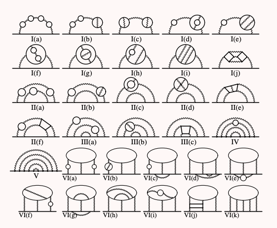
Quantum electrodynamics, or QED, covers all the possible ways a photon can interact with a muon. To get better precision, physicists can account for more virtual photons. Each additional virtual photon has about 1/137th the chance of being produced and reabsorbed, so a Feynman diagram with two virtual photons contributes about 1 / 137 * 137 to αµ, three virtual photons contribute 1 / 137 * 137 * 137, and so on. Physicists have even gone all the way to five virtual photons.
With five virtual photons, there are more than 10,000 possible paths, so there are a corresponding number of Feynman diagrams to calculate. Possibilities abound because virtual photons can split into a virtual electron and a virtual positron (the antimatter counterpart to an electron). This virtual pair can then annihilate back into a virtual photon. Describing these complex paths requires loops and squiggles that arc over each other. Five-photon Feynman diagrams look less like a traditional particle physics schematic and more like abstract art.
The weak force and the strong force
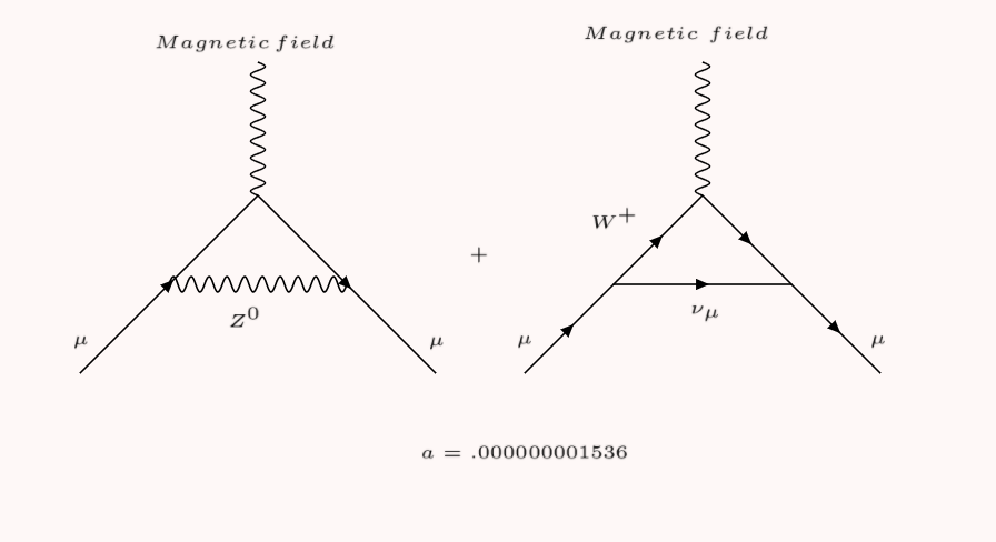
The weak force, which governs the radioactive decay of nuclei, also plays a role in influencing the muon’s magnetic moment. Unlike QED, which is mediated by the massless photon, the weak force is mediated by the massive W and Z bosons, which each weigh about 90 times the mass of a proton. The fact that the bosons are heavy makes it extremely unlikely that the muon would emit and absorb a virtual W or Z boson. But occasionally, it does happen.
Both QED and the contribution from the weak force can be calculated to extremely high precision. The process is arduous, but physicists can calculate a good deal of the interactions simply by hand. That’s not the case with contributions from particles bound together by the strong force called hadrons, which represent the majority of uncertainty in the calculation of the muon’s anomalous magnetic moment.
Gluons, the particles that mediate the strong force, are described by the rules of quantum chromodynamics, or QCD. Unlike photons in QED, gluons can interact with one another. Trying to calculate QCD processes by hand is effectively impossible, because the self-interacting gluons throw everything out of whack.
“The reason why we need a collaborative effort is because the hadronic corrections cannot be calculated from first principle QCD on a blackboard,” says El-Khadra.
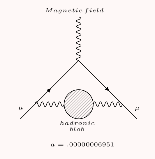
There are two main types of hadronic corrections: “vacuum polarization” corrections and “light by light” corrections. In vacuum polarization, the muon emits a virtual photon, which decays into a quark and antiquark. These quarks and antiquarks exchange gluons, turning into a frothing blob of hadronic matter such as pions and kaons. Finally, the virtual blob of hadronic matter ends when a quark and antiquark annihilate back into a virtual photon, which is finally absorbed by the muon.
Light by light contributions are perhaps some of the strangest. From the outside, it looks as if two virtual photons are emitted by a muon, interact, and are then absorbed. What’s going on here?
“When we look around us… the reason why we can see very well is because photons—to a large degree—don't interact with each other,” says Christoph Lehner, a physicist at Brookhaven National Lab and cofounder of the Theory Initiative.
But if the two virtual photons get caught in a quark loop, each converting to a virtual quark and virtual antiquark, they can form a blob of hadronic matter. If the virtual quarks and virtual antiquarks annihilate back into virtual photons, the two will appear to have bounced off of one another, interacting in a forbidden way.
Traditionally, hadronic corrections to αµ were calculated using so-called “dispersion relations.” Physicists modeling the virtual blob of hadronic matter would turn to experiments where real blobs of hadronic matter were created. Real blobs are produced in experiments where electrons collide with positrons, creating a spray of hadronic matter. Experiments like BaBar, KLOE and now Belle II all provide this kind of data, which physicists have scoured to better understand the virtual blobs.
A contribution from supercomputing
Recently, another method for calculating messy hadronic blobs has become viable, thanks to increasingly powerful computers and improved algorithms. Lattice QCD is a method for essentially simulating the blob from the ground up. Physicists write in the properties of the particles and the forces that govern them, set up a giant sandbox (a lattice) that the system can evolve in, and let it run. Lattice QCD is hugely computationally intensive—to produce a precise simulation, supercomputers have to calculate all of the gluon interchanges, a task that was impossible by hand.
Because it’s a simulation of the real world from first principles, “it’s in that sense very similar to an experiment,” according to Lehner.
One benefit is that physicists can be confident that their approach provides an answer to the question. The downsides, as in any experiment, are systematic errors—and the amount of resources required. Finding computer time is easier said than done, but at the end of the day, lattice QCD is approaching the precision of the dispersion relation method.
| Contribution | Value (x10-11) |
|---|---|
| QED | 116,584,718.931±.104 |
| Weak force | 153.6±1.0 |
| Hadronic vacuum polarization (dispersive) | 6,845±40 |
| NOT USED (Lattice hadronic vacuum polarization) | 7116±184 |
| Hadronic light-by-light (dispersive+lattice) | 92±18 |
| Total Standard Model Value | 116,591,810±43 |
| Difference from 2001 experiment | 279±76 |
Putting it all together
In February, a lattice QCD group claimed to have a result for hadronic contributions in serious conflict with the predictions of dispersive relations. Almost immediately, a flurry of other publications discussing and challenging the result followed. The June paper from the Theory Initiative does not address the potential inconsistency, but lattice QCD researchers are hard at work trying to replicate the result.
At the end of the day, when the experimentalists finish analyzing the data from the Muon g-2 experiment, they’ll compare against the theoretical value to see if there’s still a significant discrepancy. The hope, for many, is that they continue to disagree, opening a window for new physics.
Editor's note: The sentence "That's a difference of less than 3 parts per million, for those keeping score at home," has been updated to correct the number.